Algebra is generous; she often gives more than is asked of her — Jean le Rond
Before getting into Supervised learning branch of machine learning, it is imperative to get an idea about Linear algebra, followed by equation of straight line.
Linear algebra is a branch of mathematics which is concerned about linear equations. A linear equation is something which forms a line when drawn and it does have only length property, but no breadth in the mathematical space.
A form of linear equation is shown below:

The term linear equation represents an equation of first degree. We can also call the above equation as polynomial ( ‘poly’ — many and ‘nomial’ — terms) equation. When numbers are added or subtracted to the equation, they are called as terms.

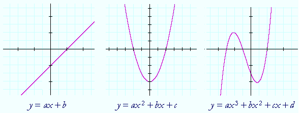
As we can see in the above picture, the graph of first degree polynomial is always a straight line , the second degree takes the shape of parabola, third degree takes the shape of a curve. Advancing with quartic, quintic polynomials, the equation becomes too complex and graph take different shapes.
The main focus point in this article is to understand that graph of any first degree polynomial is a straight line and the straight line equation can be represented as below:
y = mx + b
Here:
- y = predicted value or target variable or dependent variable
- x = independent variable or input or predictor or feature
- m = slope / weight
- b = bias / intercept
Here m and b are constants, that defines a linear relationship between x and y. The relationship between x and y is visualized as straight line and hence the term linear.
Introducing the straight line equation

When y = x, we get a straight line which passes through the origin. We can inflate y = x as below:
y = 1.x Or
y = m.x, where m = 1
Change in ‘y’ with respect to ‘x’ is represented by
𝛿y/𝛿x = Slope ( symbol delta)
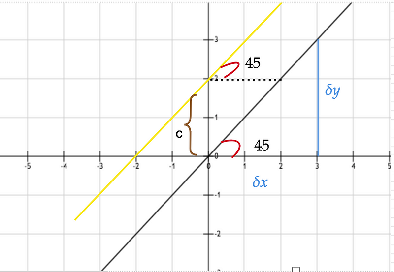
When the angle is 45 degrees ( Fig 1 ), 𝛿y/𝛿x = 1 , Since tan 𝚹 of 45 degrees = 1
The value of tan(45°) can be derived exactly by theoretical approach of geometry on the basis of a geometric property. In short ‘m’ is the tangent of the angle that the line makes with the X axis.

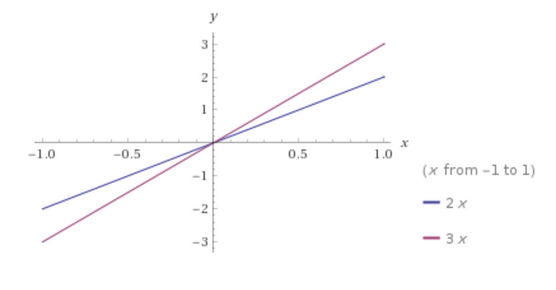
Fig 2 shows different variations of straight line equations, where the value of slope changes depending the angle.
This also represents a straight line, and for all the points on the line, each y value is three times the corresponding x value. In all the above cases the line passes through the origin.
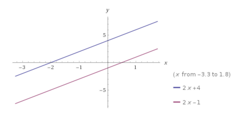
Now, look at the second line ( yellow line in Fig 1) where y is not equal to x. The line is represented by y = mx +c, where c is the intercept. When c = 0, the line passed through the origin. The number c is the point where the line cuts the y-axis.

The line is shifted either up or down depending on the value of ‘c’. If the value of the intercept is positive, the line is shifted up from the origin and vice-verse.
Conclusion
Familiarity with linear algebra, before moving into regression algorithms, would help to write custom models in Supervised learning space. The concept of the linear regression is to find a model that represents these points in the best possible way.
Do send me your comments, thoughts to Sunil Jacob.
PS: If you liked the article, please support it with claps. Cheers